Python 语言介绍
庞龙刚,华中师范大学
Life is short,use Python!
- Python 有丰富的科学计算库、可视化库
- 相比 Mathematica 和 Matlab 开源、免费、不受制裁
- 在机器学习、人工智能、量子计算领域, Python 语言有压倒性优势
- scikit-learn 机器学习
- tensorflow,pytorch 深度学习库,
Python 库的安装
- 推荐使用 Anaconda, 安装 Python 版本3.7
- 网址:https://www.anaconda.com/products/individual
- 支持 Windows,Linux,Mac 平台
- 点击前往下载链接
Python 环境管理 (初级用户可忽略)
- Windows 下使用 Anaconda Navigator
- 在用户界面管理环境和 Python 包
- 也可使用 Anaconda 中的 CMD.exe 命令行,通过 pip 安装 python 包
- Linux 下有如下系列命令,
# 查看存在的虚拟环境
 conda env list
 # 创建虚拟环境
 conda create -n your_env_name python=3.7
 # 激活虚拟环境
 conda activate your_env_name
 # 导出环境安装包
 conda env export > py37.yaml
 # 在环境中安装python库 numpy
 conda install -c conda-forge numpy
 # 退出当前环境
 conda deactivate
 # 使用导出的文件安装同样的环境
 conda env create -f py37.yaml
需要安装的库
Windows 下使用 Andconda Navigator 里的 Environments 按钮,搜索 Not installed 库安装
- numpy
- matplotlib
- pandas
- scipy
- scikit-learn
- tqdm
- h5py
- tensorflow
也可等用到时再安装。
Linux/Mac 下使用下列命令:
# 查看已经安装的Python 包
conda list
# 安装数组/矩阵操作库 numpy
conda install -c conda-forge numpy
# 安装作图库 matplotlib
conda install -c conda-forge matplotlib
# 安装大数据处理库 pandas
conda install -c conda-forge pandas
# 安装机器学习库 scikit-learn
conda install -c conda-forge scikit-learn
# 安装进程显示库 tqdm
conda install -c conda-forge tqdm

# 安装深度学习库 tensorflow (后期使用时再安装)
conda install -c conda-forge tensorflow
jupyter notebook 简单使用技巧
本课程使用 Python 的 Jupyter Notebook 交互式教学。
下载安装 Anaconda 自带 Jupyter Notebook。
- 在 jupyter notebook 中可以编辑文档,编写python程序, 键入 Latex 公式,画图,以及构造交互式工具。
- 接下来使用 jupyter notebook 简单介绍 python 语言
- Windows下在 Anaconada Navigator 中点击 Jupyter notebook 开始使用
- Linux/Mac下在命令行中键入下列命令开始使用: jupyter notebook
# jupyter-notebook cell 有两种形式,code cell 和 markdown cell
# code cell 是输入代码,按 shift+enter 运行的cell;

# markdown cell 是输入普通文字描述与 latex $\alpha + \beta = \gamma$,按 shift+enter 显示文档与数学公式的 cell
# 快捷键 m 可以快速将一个代码 cell 转化为 markdown cell

# 当前 cell 为 code cell,在 code cell 内部,# 号表示此行为注释,不进行计算
# 下一个 cell 是 markdown cell,我会输入 $ e^{2\pi i} = 1$ , 按 shift + enter 之后只显示公式

#双击公式会在 markdown cell 中显示 latex 代码
Inline formula: $ e^{2\pi i} = 1$
Eqnarray or Equation:
\begin{align} \sigma_x & = \begin{bmatrix} 0 & 1 \\ 1 & 0 \end{bmatrix} \\ \sigma_y & = \begin{bmatrix} 0 & -i \\ i & 0 \end{bmatrix} \\ \sigma_z & = \begin{bmatrix} 1 & 0 \\ 0 & -1 \end{bmatrix} \\ \end{align}点击每个 cell 左边空白,可以选中 cell
选中cell后,按 a, 可以在此 cell 上方插入一个新的 code cell
选中cell后,按 b, 可以在此 cell 下方插入一个新的 code cell
选中cell后,按 x, 可以删除此 cell
选中cell后,按 m, 可以将此 cell 转化为markdown cell
选中 markdown cell 双击,可以转化为编辑模式
基本代数运算
# Python 开箱即用,可直接进行简单计算

3 + 5
10 - 6
6 * 6
# 与 C,C++ 不同,/ 可以对两个整数相除得到浮点数
6 / 5
# 等价 C 语言中两个整数的相除
6 // 5
# 平方
31 ** 2
y = 83
z = 92
y + z
使用 math 库进行代数运算
math 是 Python 自带的一个代数运算库,里面定义了常用的 sqrt(), pow(), sin(), cos(), tan(), tanh() 等函数。
使用 dir(math) 可以打印出 math 中定义的所有函数。
import math
dir(math)
# 如果我想求一个数的阶乘,6!,但是不是很确定是否是 factorial 函数
# 此时可以用 help(math.factorial)

help(math.factorial)
# 或者把指针放在括号里,按 Shift+Tab 显示帮助文档

math.factorial(5)
import math
Test the $\sqrt{x}$ function
energy = 50
momentum = 40
mass = math.sqrt(energy**2 - momentum**2)
print(mass)
Test the pow(), which calculate $ x^m $
# 一个数的 3.5 次方
math.pow(energy, 3.5)
theta = math.pi / 6
math.sin(theta)
# 可以看到这里有截断误差,结果不严格等于 0.5
列表 list 与循环
alist = [3, 6, 'x', 3.14, [5, 9]]
alist[2]
# 一句话生成1百万个 sin(i*30度) 的列表
xlist = [math.sin(i*theta) for i in range(1000000)]
# 列表中前 10 个数, 后 10 个数,第10到第20个数

xlist[10:20]
x_sum = 0

# 注意:Python 语法的层级结构用缩紧表示
# c 语言用大括号 {}

for i in range(1000000):
    x_sum += xlist[i]

print(x_sum)
当我们对一个非常大的列表进行长时间计算时,估计大概需要的计算时间非常重要;
使用 tqdm 库,可以显示计算进程;
from tqdm import tqdm

x_sum = 0

for i in tqdm(range(10000000)):
    x_sum += 1.0E-5

print(x_sum)
使用 numba.jit 加速
python 的原始循环体比较慢,有两种方式加速,
- numpy 的 数组操作 模式
- numba 的 jit (just in time compilation 即时编译)
from numba import jit

@jit
def jit_sum():
    x_sum = 0
    for i in range(10000000):
        x_sum += 1.0E-5
    return x_sum

jit_sum()
字典类型
studentx = {'id':3300, 'score':99, 'gender':'female'}

studentx['id']
studentx['score']
for key, value in studentx.items():
    print(key, value)
集合类型
ints = set()

ints.add(3)
ints.add(5)
ints.add(7)
ints.add(3)

ints
函数 function
# 下面的介绍会用到这几个库
import numpy as np
import matplotlib.pyplot as plt
import seaborn as sns

# 画图风格与格式
sns.set_context('paper', font_scale=1.5)
sns.set_style('ticks')
# 狭义相对论
def lorentz_gamma(v):
    '''
    args:
        v: velocity over speed of the light, in [0, 1)
    return: lorentz gamma factor 1/sqrt(1-v*v)
    '''
    assert(math.fabs(v)<1.0)
    return 1/np.sqrt(1 - v*v)
lorentz_gamma(0.9999)
help(lorentz_gamma)
根据狭义相对论,
$ E = m \gamma = \frac{m}{\sqrt{1 - v^2}}$
我们来定义一个函数,计算高能核碰撞在不同能量下,原子核的飞行速度 v
# Python 函数的参数可以提供默认数值,比如此处默认 sqrtsnn=200

def velocity_of_nucleus(sqrtsnn=200):
    '''compute the velocity of nucleus given the sqrt{s_{NN}} per pair of nucleons
    args:
        sqrtsnn: the center of mass frame energy of one pair of nucleons.
        e.g., the Au+Au 200 GeV collision, each nucleon has energy 100 GeV
    return:
        the velocity of the nucleon
    '''
    energy_ = 0.5 * sqrtsnn
    nucleon_mass = 0.938
    gamma = energy_ / nucleon_mass
    velocity = math.sqrt(1 - 1/(gamma**2))
    return velocity
# 如果函数参数有默认值,可直接调用

velocity_of_nucleus()
# 也可显式赋值调用

velocity_of_nucleus(sqrtsnn=200)
# LHC 能量 sqrtsnn = 2760 GeV 碰撞
vlhc = velocity_of_nucleus(sqrtsnn=2760)
vlhc
# 在 LHC 能量下($\sqrt{s_{NN}}=2760$ GeV), 原子核被加速到了百分之 99.99998 的光速!

# 原子核沿束流方向的厚度被压缩了 1471 倍,collision of pancakes!

lorentz_gamma(vlhc)
递归函数(数学中归纳法)
- 已知 n = 1 时结果
- 知道 n 到 n+1 的递推公式
例子:勒让德多项式
$$P_0(x) = 1, \quad\; P_1(x) = x,\quad\; P_{n+1}(x) = \left[ (2n+1) x P_n(x) - n P_{n-1} (x)\right]/(n+1) $$def Pn(x, n):
'''此处,Pn 是递归函数,需要调用自己计算 Pn(n-1) 与 Pn(n-2)'''
if n == 0:
return np.ones_like(x)
elif n == 1:
return x
else:
return ((2*n-1)*x*Pn(x, n-1) - (n-1)*Pn(x, n-2))/n
x = np.linspace(0, 1, 100)

for n in range(5):
    legi = Pn(x, n)
    plt.plot(x, legi, label="%s"%n)
    plt.xlabel("x")
    plt.ylabel(r"$P_n(x)$")
    plt.legend(loc="best")

Warning 警告:如果将数组作为函数的参数输入,可能会以奇怪的方式改变数组的数值!
如果不是用 copy 函数,列表作为参数时传递的是数组的地址!
alist = [3, 4, 5, 6]

def test_func(list_arg):
    blist = list_arg
    blist.append(7)
    #print(blist)

test_func(alist)

print(alist)
alist = [3, 4, 5, 6]

def test_func(list_arg):
    # 如果不想改变list参数,用 copy 函数
    blist = list_arg.copy()
    blist.append(7)
    print("blist=", blist)

test_func(alist)

print("alist=", alist)
面向对象编程:类(Class)
class Particle:
    def __init__(self, mass, spin, isospin):
        self.mass = mass
        self.spin = spin
        self.isospin = isospin

    def spin_degenaracy(self):
        '''return: the spin degenaracy of the particle'''
        return 2*self.spin + 1

    def is_fermion(self):
        '''check whether a particle is fermion or boson'''
        g = self.spin_degenaracy()
        if g%2 == 0:
            return True
        else:
            return False

    def thermal_distribution(self, momentum, T):
        '''Args:
              T: the temperature of the medium
           return:
              the fermion dirac or boson-eistein distribution'''
        assert(T>0)
        E = np.sqrt(momentum**2 + self.mass**2)
        if self.is_fermion():
            dist = self.spin_degenaracy() / (np.exp(E/T) + 1)
        else:
            dist = self.spin_degenaracy() / (np.exp(E/T) - 1)
        return dist
pion = Particle(mass=0.138, spin=0, isospin=1)
pion.is_fermion()
momentum = np.linspace(0.1, 3, 20)
density = pion.thermal_distribution(momentum, T=0.137)
print(density)
kaon = Particle(mass=0.49, spin=0, isospin=1)
kaon_density = kaon.thermal_distribution(momentum, T=0.137)
plt.semilogy(momentum, density)
plt.semilogy(momentum, kaon_density, 'o-')

读写文件操作
最常用的文件格式:txt, csv, hdf5
- csv 是 txt 类型数据格式 (交互性较好)
- hdf5 是二进制类型数据格式 (数据载入速度比较快)
- 少量数据用 txt,大量数据用 hdf5
下面介绍几种文件读写方法。
1. 使用 python 系统 io 进行 txt 文件读写
with open("test.txt", "w") as fout:
    fout.write("hello world")
这条命令打开一个文件 test.txt, 向其中写入 "hello world", 并关闭文件。
使用 with 语句可以保证在读写文件失败的时候,文件自动关闭,推荐使用。
# 打开文件,向其中写 hello world
with open("test.txt", "w") as fout:
    fout.write("hello world")

# 此时可以检查,目录下多了 test.txt
# !cat 是命令行工具,可以输出文件内容
!cat test.txt
#  读文件,并输出
with open("test.txt", "r") as fin:
    txt = fin.read()

print("Read from test.txt :", txt)
# 产生 5 行 4 列 随机数,范围 [0, 1)
rand_data = np.random.rand(5, 4)

rand_data
# 保存数据到硬盘

np.savetxt("rand_data.txt", rand_data)

!cat rand_data.txt
# 从硬盘文件 rand_data.txt 读取数据
mydata = np.loadtxt("rand_data.txt")
mydata
3. 使用 pandas 读写文件
pandas 可以读取 csv、excel、hdf5、json、xml 等文件格式
这里仅对 csv 格式文件进行示例。
这里需要先产生 DataFrame 类型数据,然后对其进行保存。
import pandas as pd

df = pd.DataFrame(data=mydata,
                  columns=['col1', 'col2', 'col3', 'col4'])

# pandas 的 DataFrame 多存储了每一列的名字
df.to_csv("pd_data.csv")

!cat pd_data.csv
pd_data = pd.read_csv("pd_data.csv", index_col=0)

pd_data.head()
import h5py

# 将数据写入文件,可以使用 create_dataset 创建多个 dataset
with h5py.File("h5_file.h5", "w") as h5:
    h5.create_dataset("rand", data=mydata)

# 从 h5 文件中读取数据,h5["rand"][...] 将其表示为 numpy 数组
with h5py.File("h5_file.h5", "r") as h5:
    h5data = h5["rand"][...]

print(h5data)
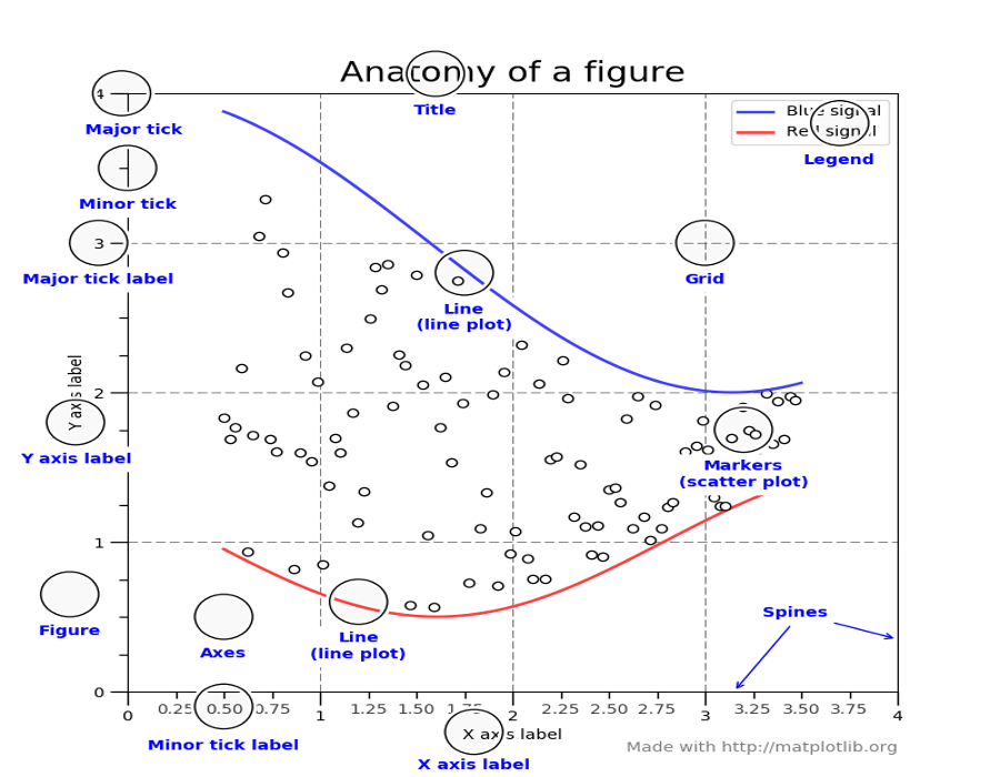
Python 画图 (科学绘图中不同对象的名称)
# matplotlib 绘图:先产生离散的坐标 x,区间[-10, 10], 100 个点
x = np.linspace(-10, 10, 100)
# 再计算这些坐标上的 y,使用 numpy 函数可以直接操作整个数组中的所有元素
y = np.sin(x)
# 画出红色的点线图
plt.plot(x, y, 'ro-')

plt.xlabel("x")
plt.ylabel("$\sin(x)$")
plt.savefig("sinx.pdf")

# Legend for different lines

x = np.linspace(-10, 10, 100)
y = np.sin(x)

plt.plot(x, np.sin(x), 'o', label='y=sin(x)')
plt.plot(x, np.cos(x), 'o-', label='y=cos(x)')

plt.xlabel("x")
plt.ylabel("y")
plt.legend(loc='best')
#plt.savefig("legend.pdf")

# 适合文章发表要求的图片格式, 使用 SciencePlots 库
# pip install SciencePlots
def pretty_plot():
    with plt.style.context(['science','ieee', 'no-latex']):
        x = np.linspace(-10, 10, 100)
        y = np.sin(x)

        plt.plot(x, np.sin(x), label='y=sin(x)')
        plt.plot(x, np.cos(x), label='y=cos(x)')

        plt.xlabel("x")
        plt.ylabel("y")

        # change y range
        plt.ylim(-1.5, 2.5)
        plt.legend(loc='best')
        #plt.savefig("legend.pdf")
pretty_plot()

简单的交互
y = 8
# 简单的猜数游戏
x = int(input("输入你猜的数:"))

while x != y:
    if x < y:
        x = int(input("猜小了,请重猜:"))
    elif x > y:
        x = int(input("猜大了, 请重猜:"))

print("猜对了!")
# 需要安装 ipywidgets 插件

from ipywidgets import interact

@interact(m=10, b=10)
def plot_line(m, b):
    print('%s * x + %s'%(m, b))
@interact(m=1, b=1)
def plot_line(m, b):
    x = np.linspace(-10, 10, 100)
    plt.plot(x, m*x + b)
    plt.xlim(-10, 10)
    plt.ylim(-10, 10)
如何开发自己的 Python 模块、库
如果想在 jupyter notebook 或其他 python 文件中 import 自己的库,
可以使用自己喜欢的文本编辑器,将代码存放在自己命名的 mylib.py 文本文件中,然后直接导入:
import mylib
# mylib.py 中的内容,除了变量定义,函数定义以及类定义之外,还可以包含 main() 函数,测试时使用。

# 比如,将下面内容写入文件 test.py, 再 import test 库

source_code = '''
#!/usr/env python

import numpy as np

def azimuthal_angle(px, py):
    return np.arctan2(py, px)

if __name__ == "__main__":
    phi = azimuthal_angle(4, 4)
    print("phi=", phi)
'''

with open("test.py", "w") as fout:
    fout.write(source_code)
!cat test.py
!python test.py
import test

# 可以看到 if __name__ == "__main__" 之后的代码只有在直接运行时起作用
# 作为库使用时,不会导入

test.azimuthal_angle(px=3, py=5)
Python 语法中比较难理解的两点(知道即可)
- Generator 生成器
- Decorator 装饰器
Generator 举例: range(n) 其实是生成器,在
for i in range(10000): 语句中,
它并不直接生成并保存一个超大数组,而是从 i=0 开始,一个个生成。
所以,range(10) 并不能当做数组 $[0, 1, 2, \cdots, 9]$ 用。
# 此处可以看出,range(10) 是一个 generator
range(10)
# 只有加 list() 才会显式计算,并将 generator 转化为 list
list(range(10))
# generator 用 yield 语法实现
def myrange(n=10):
    '''range 的实现'''
    i = 0
    while i < n:
        # yield 调用后会暂停
        yield "my element: %s"%i
        i = i + 1

myrange(10)
# yield 保证需要用到时方生成
for i in myrange(5):
    print(i)
# 举例:hello 是函数的函数
def hello(func_username):
    '''输入、输出皆为函数'''
    def inner(s):
        return "hello %s"%func_username(s)

    return inner

def username(s):
    return s

username("Alice")
hello_user = hello(username)
hello_user("Alice")
# 语法糖:将 hello 装饰在 username 上
# 与 hello(username)("Bob") 等价
@hello
def username_(s):
    return s

username_("Bob")
大型的计算物理程序编写原则
- 自顶向下,先规划好程序结构,将不同的功能模块化、函数化
- 每个模块可分离,并对每个模块做尽可能多的单元测试(unit tests)
- 模块、类、函数命名规范,并有清晰的说明文档 help(func)
- 对给定的物理问题,在简化假设下,对比数值解与解析解
- 检查守恒律,比如能量、动量、净电荷守恒、细致平衡等
- 如果市面上有其他代码,与其他代码结果做对比