使用数值积分计算理想强子共振气体的状态方程
庞龙刚@华中师范大学
学习目标
- 数值积分在真实物理研究中应用
- 认识强子、理想强子共振气体、状态方程
学习内容
- 什么是强子
- 高能核碰撞末态强子的统计分布
- 从粒子数据表 pdg data table 中读取各种强子的量子数
- 计算所有强子对强子共振气体状态方程的贡献
import numpy as np
import matplotlib.pyplot as plt

# quad 函数用来做数值积分
from scipy.integrate import quad

import seaborn as sns

sns.set_context("talk")
强子共振气体 (Hadron Resonance Gas: HRG)
美国布鲁克海文国家实验室的相对论重离子碰撞机RHIC,以及欧洲核子中心的大强子对撞机LHC上进行的重离子碰撞实验(比如剥离核外电子的金核+金核、铅核+铅核碰撞)产生了解禁闭的夸克胶子等离子体(QGP:Quark Gluon Plasma),QGP 冷却后生成大量强子,这些强子经历散射、共振产生以及衰变的一系列过程。
- 强子:包括介子(Meson)与重子(Baryons)
- 介子:由一个 quark + 一个反 quark + 胶子组成的束缚态,比如 pion 介子(夸克组分 $u\bar{d}$)
- 重子:由3个夸克(或反夸克)+胶子组成的束缚态,比如质子(uud), 中子(udd), Lambda (uds)等等
从 https://pdg.lbl.gov/ 可以查到目前发现的所有强子的数据。
%%HTML
<div align="middle">
<video width="80%" controls>
      <source src="images/smash_movie.mp4" type="video/mp4">
</video>
</div>
# 这类动画使用 Paraview 制作。将程序运行结果保存为 VTK 格式,然后输入 Paraview 可视化
粒子产额与参考系无关,可以使用局域静止参考系(随动系),此时强子的动量分布各向同性 $\int d^3 p = \int 4\pi p^2 dp$, 强子的统计产额与温度 T、强子质量 m、强子自旋 s 的关系为,
\begin{align} f(T) = (2 s + 1) \int {4\pi p^2 dp\over (2\pi)^3} {1 \over e^{\sqrt{p^2 + m^2} \over T} \pm 1} \end{align}强子如 pion 介子、kaon(K介子)、proton(质子)的质量、自旋、种类(玻色子或费米子)可以通过查 PDG data table 得到。
强子产额的计算化为对动量的一维数值积分,此产额又称统计产额,积分计算结果与高能核碰撞实验得到的末态强子产额基本一致。
强子共振气体的状态方程
状态方程 (Equation of state) 描述了大量粒子(宏观)的统计性质,比如系统的能量密度,温度,压强,熵密度之间的关系等等。
这里,根据统计力学公式,计算如下量,
- 零质量理想气体的状态方程 (P = e/3)
- 理想 pion 介子气体的状态方程 (P < e/3)
- 理想 强子共振气体的状态方程 (P ~ e/6)
理想气体:粒子之间只存在弹性散射
统计学公式: Interacting hadron resonance gas meets lattice QCD
第 i 种强子的巨正则配分函数,
\begin{align} \ln Z_i^{id gas} = \pm {V g_i \over 2 \pi^2} \int_0^{\infty} k^2 dk \ln \left[ 1 \pm exp(-(E_i - \mu_i)/T \right] \end{align}- $g_i=(2s+1)$ 是自旋简并度
- 对于重子,取 $+$,统计分布为 Fermi-Dirac 分布
- 对于介子,取 $-$, 统计分布为 Bose-Einstein 分布
- $\mu_i$ 是第 i 种强子的化学势
化学势
化学势保证了统计意义上系统的净重子数、净奇异数(s quark - anti s quark 对称)、净电荷数守恒。
\begin{align} \mu_i = b_i \mu_B + s_i \mu_S + q_i \mu_Q \end{align}$b_i,s_i,q_i$ 是第 i 种强子对应的重子数、奇异数和电荷数,从 PDG table 可以查到。
- 净重子数守恒:$ V\sum_i n_i b_i = N_B$
- 净电荷数守恒:$ V\sum_i n_i q_i = N_Q$
- 净奇异数守恒:$ V\sum_i n_i s_i = N_S$
其中 $n_i$ 是第 i 种强子的密度,$N_B, N_Q, N_S$ 分别是系统的净重子数,净电荷数,净奇异数。
在中低能核碰撞中,入射核与靶原子核中的质子和中子使得能量沉积区域正物质多于反物质,导致
- 净重子数不为 0,
- 净电荷(质子)不为 0,
- 净奇异数仍为 0
化学势的存在使得正物质本身不需要守恒,反物质本身也不需要守恒,但是正反物质的差、正负电荷的差必须守恒。
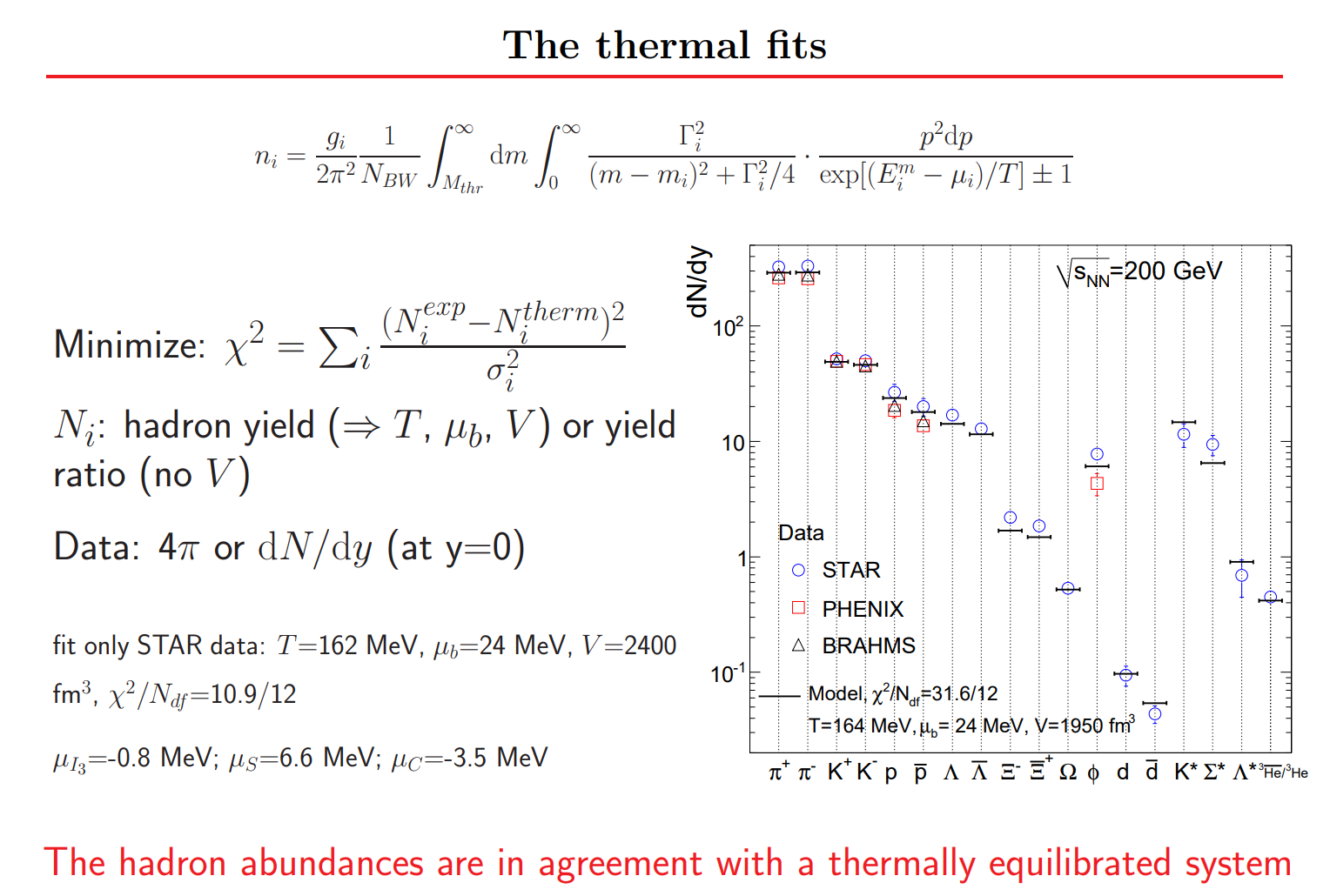
给定 $\mu_B$, $\mu_S$, $\mu_Q$, 温度 $T$ 以及体积 $V$ 可以确定第 i 种强子的产额,以及总的 $N_B, N_Q, N_S$;
现实中反过来,给定实验数据,拟合 $\mu_B$, $\mu_S$, $\mu_Q$, 温度 $T$ 以及体积 $V$。
从真空中激发出的粒子正物质与反物质对称,
- 净重子数 $N_B = 0$
- 净电荷数 $N_Q = 0$
- 净奇异数 $N_S = 0$
高能核碰撞以及宇宙早期图像都产生了等量的正反物质,重子化学势、奇异化学势、电荷化学势都很小。
强子共振气体的压强 pressure 和能量密度 energy density 由下面两个统计学公式给出,其中 $\sum_i$ 对所有强子求和
\begin{align} p(T, \mu) &= \sum_i {T \ln Z_i^{id gas} \over V } = \sum_i \pm {T g_i \over 2 \pi^2} \int_{0}^{\infty} k^2 dk \ln \left[ 1 \pm exp(-(E_i - \mu_i)/T \right] \\ \varepsilon(T, \mu) &= - \sum_i {1 \over V }\left( {\partial \ln Z_i^{id gas} \over \partial (1/T)} \right)_{1 / \mu_i} \\ & =\sum_i {2s + 1 \over 2 \pi^2} \int_{0}^{\infty} {k^2 dk \sqrt{k^2 + m^2}} \left[\exp\left(\sqrt{k^2 + m^2} - \mu_i \over T \right) + \eta_i\right]^{-1} \end{align}根据压强与能量密度,可以定义声速的平方,
\begin{align} c_s^2 = {d P \over d \varepsilon} \end{align}声速反应扰动在介质中传播的速度。
声速 (Speed of sound)
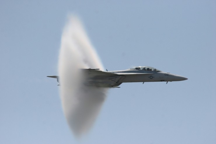
超音速飞机在波前会形成马赫锥 (Mach Cone), 马赫锥的角与声速的关系为,
\begin{align} \sin {\theta \over 2} = {c_s \over v_{\rm jet}} \end{align}使用高能部分子(喷注)穿过 QGP 时的行为可以研究夸克胶子等离子体的状态方程(声速)。
此外,核物质的状态方程有很多其他用途,比如
使用相对论流体力学模拟 QGP 时空演化时,状态方程至关重要,因为 QGP 膨胀的驱动力是压强梯度 $-dP/dx$
中子星的质量半径关系由核物质状态方程决定(参考:Tolman-Oppenheimer-Volkoff (TOV) equation)
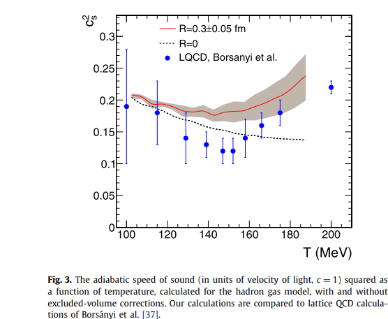
Interacting hadron resonance gas meets lattice QCD 文章截图,(R=0 强子共振气体与 Lattice QCD 状态方程非常接近)
第一种简化假设:只考虑 pion 介子
- 质量:m=135$\sim$139 MeV
- 自旋:s= 0
- 玻色子:$\eta_i$ = -1
- 化学势 $\mu \equiv (\mu_B, \mu_S, \mu_Q) = (0, 0, 0)$ 。
即构造一个简单的状态方程,对应宇宙早期和高能核碰撞,考虑压强、能量密度与温度的关系
pion0 = {'mass': 0.135,    # unit: [GeV]
        '2*spin+1': 1,     # spin degeneracy
        'eta': -1,         # - for boson
        'baryon_num': 0,
        'strange_num': 0,
        'charge_num': 0}
def dist_f(k, T, hadron):
    '''the distribution function of hadron
    :k: float or np.array(), momentum in units [GeV]
    :T: float, temperature, [GeV]
    :hadron: dict with {'mass', '2*spin+1', 'eta',
                        'baryon_num', 'strange_num', 'charge_num'}
             where eta: +1 for fermion, -1 for boson

    :return: (2s + 1) / (np.exp(np.sqrt(k**2 + m**2)/T) + eta)
    '''
    spin_dof = hadron['2*spin+1']
    m = hadron['mass']
    eta = hadron['eta']
    return  spin_dof / (np.exp(np.sqrt(k**2 + m**2)/T) + eta)
def density_n(T, hadron):
    '''calc density for given temperatures
    :T: float, temperature, [GeV]
    :hadron: dict with {'mass', '2*spin+1', 'eta',
                        'baryon_num', 'strange_num', 'charge_num'}
             where eta: +1 for fermion, -1 for boson
    :return: hadron density at T '''
    # 此处 intg_n 是 inline function
    intg_n = lambda k: k**2 * dist_f(k, T, hadron) / (2 * np.pi**2)

    kmax = 50 * T
    # 不要直接使用 quad(f, 0, 50*T), 给 50*T 命名为 kmax,程序可读性更好
    ndensity = quad(intg_n, 0, kmax)[0]

    return ndensity
# 高能核碰撞产生大量强子中,pion 介子占 80% 以上,可以从 pion/proton ratio 简单看出
proton = {'mass': 0.938,    # unit: [GeV]
        '2*spin+1': 2,
        'eta': +1,
        'baryon_num': 1,
        'strange_num': 0,
        'charge_num': 1}

T = 0.155
npi0 = density_n(T, pion0)
nproton = density_n(T, proton)

print("pion to proton ratio=", npi0 / nproton)
def pressure_p(T, hadron):
    '''HRG presure for given temperatures
    :T: float or np.array(), temperature, [GeV]
    :hadron: dict with {'mass', '2*spin+1', 'eta',
                        'baryon_num', 'strange_num', 'charge_num'}
             where eta: +1 for fermion, -1 for boson
    :return: hadron presure at T  in unit [GeV]^4 '''
    spin_dof = hadron['2*spin+1']
    m = hadron['mass']
    eta = hadron['eta']
    intg_p = lambda k:  k**2 * np.log(1 + eta * np.exp(-(np.sqrt(k**2 + m**2))/T))
    coef_p = eta * T * spin_dof / (2 * np.pi**2)

    kmax = 50 * T
    pressure = coef_p * quad(intg_p, 0, kmax)[0]
    return pressure
def energy_density_e(T, hadron):
    '''HRG presure for given temperatures
    :T: float or np.array(), temperature, [GeV]
    :hadron: dict with {'mass', '2*spin+1', 'eta',
                        'baryon_num', 'strange_num', 'charge_num'}
             where eta: +1 for fermion, -1 for boson
    :return: hadron energy density at T in unit [GeV]^4'''
    m = hadron['mass']

    intg_e = lambda k: k**2 * np.sqrt(k**2 + m**2) * dist_f(k, T, hadron) / (2 * np.pi**2)
    kmax = 50 * T
    edensity = quad(intg_e, 0, kmax)[0]
    return edensity
def eos(T, mu, hadron):
    '''calc the pressure vs energy density
    :T: float, temperature, [GeV]
    :mu: (mu_B, mu_S, mu_Q)
    :hadron: dict with {'mass', '2*spin+1', 'eta',
                        'baryon_num', 'strange_num', 'charge_num'}
             where eta: +1 for fermion, -1 for boson
    return: pressure, energy density in unit [GeV]^4,particle density'''
    pressure = pressure_p(T, hadron)
    edensity = energy_density_e(T, hadron)
    ndensity = density_n(T, hadron)

    return pressure, edensity, ndensity
无质量理想气体状态方程
\begin{align} P = {\varepsilon \over 3} \end{align}下面我们定义一个虚假的强子 $mass=0$, 测试数值计算出的状态方程是否满足 $P = {\varepsilon \over 3}$.
# 测试无质量理想气体的状态方程 P = e/3

fake_hadron = {'mass': 0,  # unit: [GeV]
        '2*spin+1': 1,     # spin degeneracy
        'eta': -1,         # - for boson
        'baryon_num':  0,
        'strange_num': 0,
        'charge_num': 0}

Tarr = np.linspace(0.01, 0.2, 100)

ed = [energy_density_e(T, fake_hadron) for T in Tarr]

pr = [pressure_p(T, fake_hadron) for T in Tarr]

np.isclose(np.array(pr), np.array(ed)/3).all()
def plot_pr_vs_ed(ed, pr, label="EoS for massless ideal gas"):
    with plt.style.context(["science", "notebook", "no-latex"]):
        plt.plot(ed, pr, label=label)
        plt.xlabel(r"energy density ${\rm [GeV]^{-4}}$")
        plt.ylabel(r"pressure ${\rm [GeV]^{-4}}$")
        plt.legend(loc='best')

plot_pr_vs_ed(ed, pr)

$\pi$ 介子气体
$\pi^0$ 质量约为 0.135 GeV,自旋为 0,其压强与能量密度的关系是否满足 $P = {\varepsilon \over 3}$?
pion_ed = [energy_density_e(T, pion0) for T in Tarr]

pion_pr = [pressure_p(T, pion0) for T in Tarr]

np.isclose(np.array(pion_pr), np.array(pion_ed)/3).all()
with plt.style.context(["science", "notebook", "no-latex"]):
    plot_pr_vs_ed(pion_ed, pion_pr, label="pion0 gas")
    plt.plot(ed, np.array(ed)/3.0, 'r--', label="massless ideal gas")
    plt.legend(loc='best')

cs2_pion = np.gradient(pion_pr, pion_ed)

with plt.style.context(["science", "notebook", "no-latex"]):
    plt.plot(Tarr, np.ones_like(Tarr)/3, label="mass less ideal gas")
    plt.plot(Tarr, cs2_pion, label="pion0 gas")
    plt.legend(loc='best')
    plt.xlabel('T [GeV]')
    plt.ylabel(r'$c_s^2$')

Pion + Proton 气体
如果系统不是单一的 pion 介子气体,而是介子与质子的混合气体呢?
# HRG with pion and proton only

def simple_hrg_eos():
    T = np.linspace(0.05, 0.350, 100)
    mu = 0
    pressure = []
    edensity = []
    cs2 = []

    for Ti in T:
        pr_pion, ed_pion, n_pion = eos(Ti, mu, pion0)
        pr_proton, ed_proton, n_proton = eos(Ti, mu, proton)
        pr_ = pr_pion + pr_proton
        ed_ = ed_pion + ed_proton
        pressure.append(pr_)
        edensity.append(ed_)

    cs2 = np.gradient(pressure, edensity)

    return T, pressure, edensity, cs2
T, pre, ed, cs2 = simple_hrg_eos()
plt.plot(T, pre, label="p(T)")
plt.plot(T, ed, label="ed(T)")
plt.legend(loc='best')
plt.xlabel('T')

plt.plot(ed, pre, label="p(ed)")
plt.legend(loc='best')
plt.xlabel('ed')

plt.plot(T, cs2, label="pion+proton")
plt.plot(Tarr, cs2_pion, label="pion0 gas")
plt.xlabel("Temperature [GeV]")
plt.ylabel(r"$c_s^2$")
plt.legend(loc='best')

- pion0 介子与质子混合气体的状态方程与 HRG 的状态方程有不小差距
- 但加入更多强子时,声速平方小于无质量理想气体的 $1/3$,并且越来越小
- 下面考虑加入更多强子,看是否能得到与 Lattice QCD 相近的结果
HRG EoS using PDG05 table
PDG05 table 使用 05 年的 PDG 数据,数字化后保存了介子与重子(注意没有反重子)的量子数以及衰变分支信息。
pdg_ = []
name_ = []
mass_ = []
decay_width_ = []       # decay width
spin_degeneracy_ = []    # 2*s + 1
isbaryon_ = []
strange_num_ = []
charge_num_ = []
with open("data/pdg05.dat", "r") as pdg:
    lines = pdg.readlines()
    row = 0
    while row < len(lines):
        # 按空格将不同的数据分开
        particle = lines[row].split()
        # 最后一列存储了衰变通道个数
        decay_channels = int(particle[-1])
        row += decay_channels

        #print(particle[1], particle[10])
        pdg_.append(int(particle[0]))
        name_.append(particle[1])
        mass_.append(float(particle[2]))
        decay_width_.append(float(particle[3]))
        spin_degeneracy_.append(int(particle[4]))
        isbaryon_.append(int(particle[5]))
        strange_num_.append(int(particle[6]))
        charge_num_.append(int(particle[10]))

        row += 1
import pandas as pd

df = pd.DataFrame({"pdg":pdg_,
                   "name":name_,
                   "mass":mass_,
                   "decay_width":decay_width_,
                   "2*spin+1":spin_degeneracy_,
                   "isbaryon":isbaryon_,
                   "strange_num":strange_num_,
                   "charge_num":charge_num_})
df.head(n=10)
# 给 pandas 的 DataFrame 数据多添加一列,eta

# for fermions (baryons)
df.loc[df["isbaryon"]==1, "eta"] = +1.0

# for bosons (mesons)
df.loc[df["isbaryon"]==0, "eta"] = -1.0
# pdg05.dat 中无反重子,手动添加
anti_baryon = df[df['isbaryon']==1].copy()
anti_baryon.loc[:, "pdg"] = - anti_baryon["pdg"]
anti_baryon.loc[:, "name"] = "anti" + anti_baryon["name"]
anti_baryon.loc[:, "charge_num"] = -anti_baryon["charge_num"]
anti_baryon.head()
df = df.append(anti_baryon, ignore_index=True)
df.tail()
df.count()['pdg']
使用 PDG05 table,计算理想强子共振气体的状态方程
from tqdm import tqdm

# HRG with pion and proton only

def hrg_eos():
    T = np.linspace(0.1, 0.2, 20)
    mu = 0
    pressure = []
    edensity = []
    ndensity = []
    cs2 = []

    for Ti in tqdm(T):
        pr = 0
        ed = 0
        nd = 0
        for i in range(len(df)):
            hadron = df.iloc[i, :]
            pr_, ed_, nd_ = eos(Ti, mu, hadron)
            pr += pr_
            ed += ed_
            nd += nd_

        pressure.append(pr)
        edensity.append(ed)
        ndensity.append(nd)

    cs2 = np.gradient(pressure, edensity)

    return T, np.array(pressure), np.array(edensity), np.array(ndensity), cs2
T, Pr, Ed, Nh, Cs2 = hrg_eos()
plt.plot(T, Cs2)
plt.xlabel("T [GeV]")
plt.ylabel(r"$c_s^2$")

plt.plot(Ed, Pr)
plt.xlabel(r"$\varepsilon\ [GeV]^4$")
plt.ylabel(r"$P\ [GeV]^4$")

plt.plot(T, Ed/T**4)
plt.xlabel("T [GeV]")
plt.ylabel(r"$\varepsilon / T^4$")

plt.plot(T, 3 * Pr/T**4)
plt.xlabel("T [GeV]")
plt.ylabel(r"$3 P / T^4$")

to_fm_3 = (1/0.19732)**3
plt.plot(T, np.array(Nh) * to_fm_3)
plt.ylim(0, 1.4)
plt.xlabel("T [GeV]")
plt.ylabel(r"Hadron density $fm^{-3}$")

作业:
- 使用 WebplotDigitizer 从文章 Interacting hadron resonance gas meets lattice QCD 的 Fig.1, Fig. 3, Fig. 4 中提取 Lattice QCD 计算结果,并与上面计算结果画在同一张图中,作为对比(添加 xlabel,ylabel,legend)。